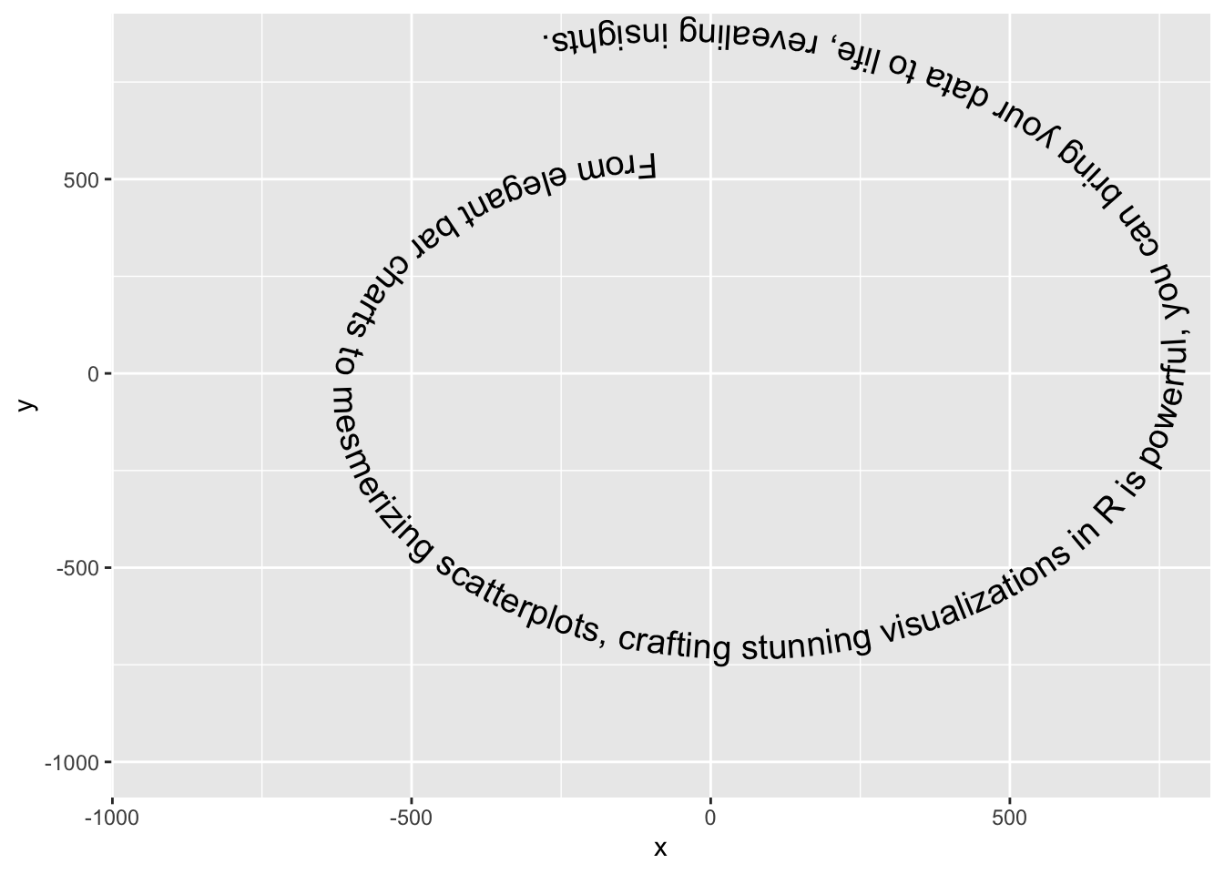
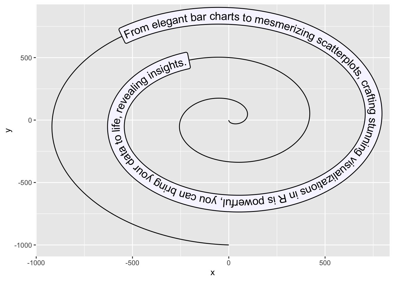
Beautiful Plots with Texts with geomtextpath


This post explains how to create plots with texts or to combine chart and text in your ggplot2 plots using the geomtextpath package.
This post showcases the key features of geomtextpath and provides a set of graph examples using the package.

Documentation

{geomtextpath}

Quick start


The geomtextpath package in R is an extension of the ggplot2 package, designed to simplify the process of adding text in charts, especially when you need the text to follow a curved path.

It offers a set of functions inspired by ggplot2, with the advantage of making it much easier to add text following a (curved) path.

✍️ author → Allan Cameron

📘 documentationgithub

⭐️ more than 500 stars on github

Installation


To get started with geomtextpath, you can install it directly from CRAN using the install.packages function:

install.packages("geomtextpath")

Basic usage


The geomtextpath package needs the x and y coordinates, the label, and you’re good to go!

To keep in mind: in function names, you can change the text to label (and vice versa) to choose whether the text should be framed or not.

Here’s a basic example:

library(ggplot2)
library(geomtextpath)

t = seq(5, -1, length.out = 1000) * pi
spiral = data.frame(x    = sin(t) * 1:1000, 
                    y    = cos(t) * 1:1000,
                    text = paste("From elegant bar charts to mesmerizing scatterplots,",
                                 "crafting stunning visualizations in R is powerful,",
                                 "you can bring your data to life, revealing insights.")
                     )

ggplot(spiral, aes(x, y, label = text)) +
  geom_textpath(size = 5, vjust = 1, text_only = TRUE)

Key features


→ Text in a box

You can have the text in a box thanks to the geom_labelpath() function.

Example:

ggplot(spiral, aes(x, y, label = text)) + 
  geom_labelpath(size = 5, fill = "#F6F6FF", hjust = 0.55)

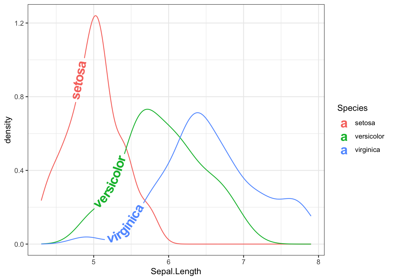
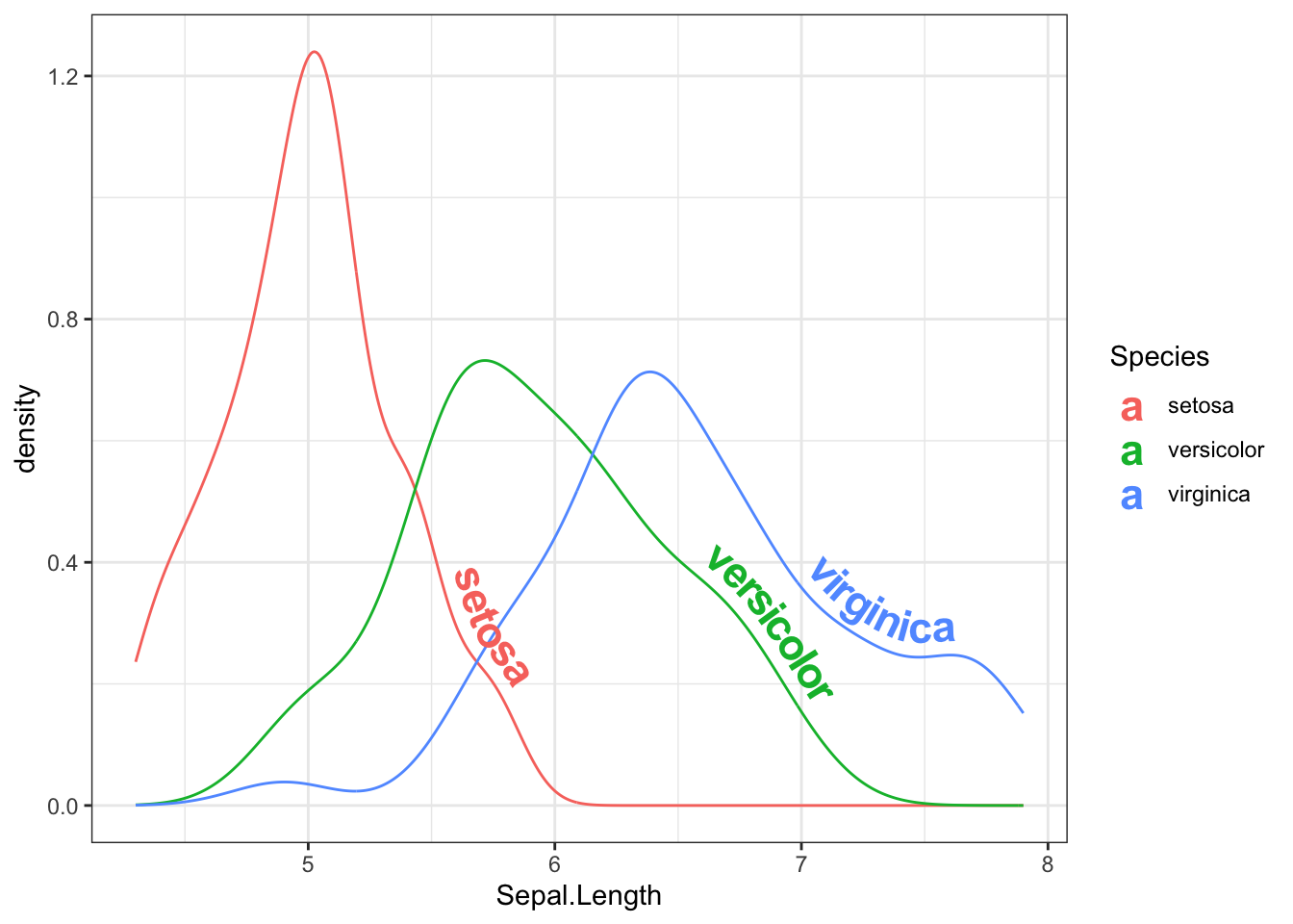
→ Text on density chart

The geom_textdensity() can be used to plot group name directly on the curve of a density chart. You can adjust the position of the text with the vjust and hjust arguments (numerical value or “xmid”/“ymax”/“auto”).

Example with the iris dataset:

library(hrbrthemes)
data(iris)

ggplot(iris, aes(x = Sepal.Length, colour = Species, label = Species)) +
  geom_textdensity(size = 6, fontface = 2, vjust = -0.4, hjust = "ymid") +
  theme(legend.position = "none") + theme_bw()

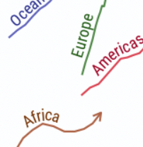
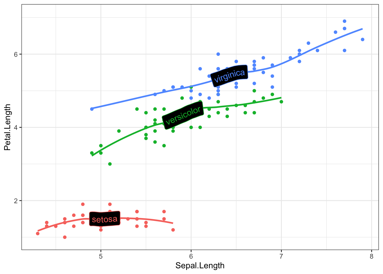
→ Labelled trend lines

You can add trend lines with the group label on top with the geom_labelsmooth() function

Example:

data(iris)

ggplot(iris, aes(x = Sepal.Length, y = Petal.Length, color = Species)) +
  geom_point() +
  geom_labelsmooth(aes(label = Species), fill = "black",
                method = "loess", formula = y ~ x,
                size = 4, linewidth = 1, boxlinewidth = 0.3) +
  theme_bw() + guides(color = 'none') # remove legend
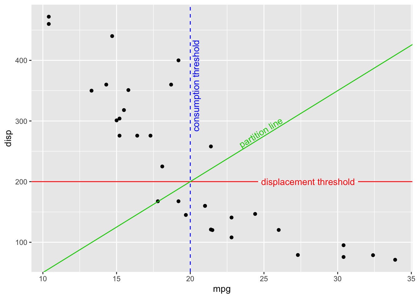
→ Reference lines

You can add reference lines with your own label thanks to the geom_texthline(), geom_textvline() and geom_textabline() functions.

Example:

data(mtcars)

ggplot(mtcars, aes(mpg, disp)) + 
  geom_point() + 
  geom_texthline(yintercept = 200, label = "displacement threshold", 
                 hjust = 0.8, color = "red") +
  geom_textvline(xintercept = 20, label = "consumption threshold", hjust = 0.8,
                 linetype = 2, vjust = 1.3, color = "blue") +
  geom_textabline(slope = 15, intercept = -100, label = "partition line", 
                  color = "green3", hjust = 0.6, vjust = -0.2)

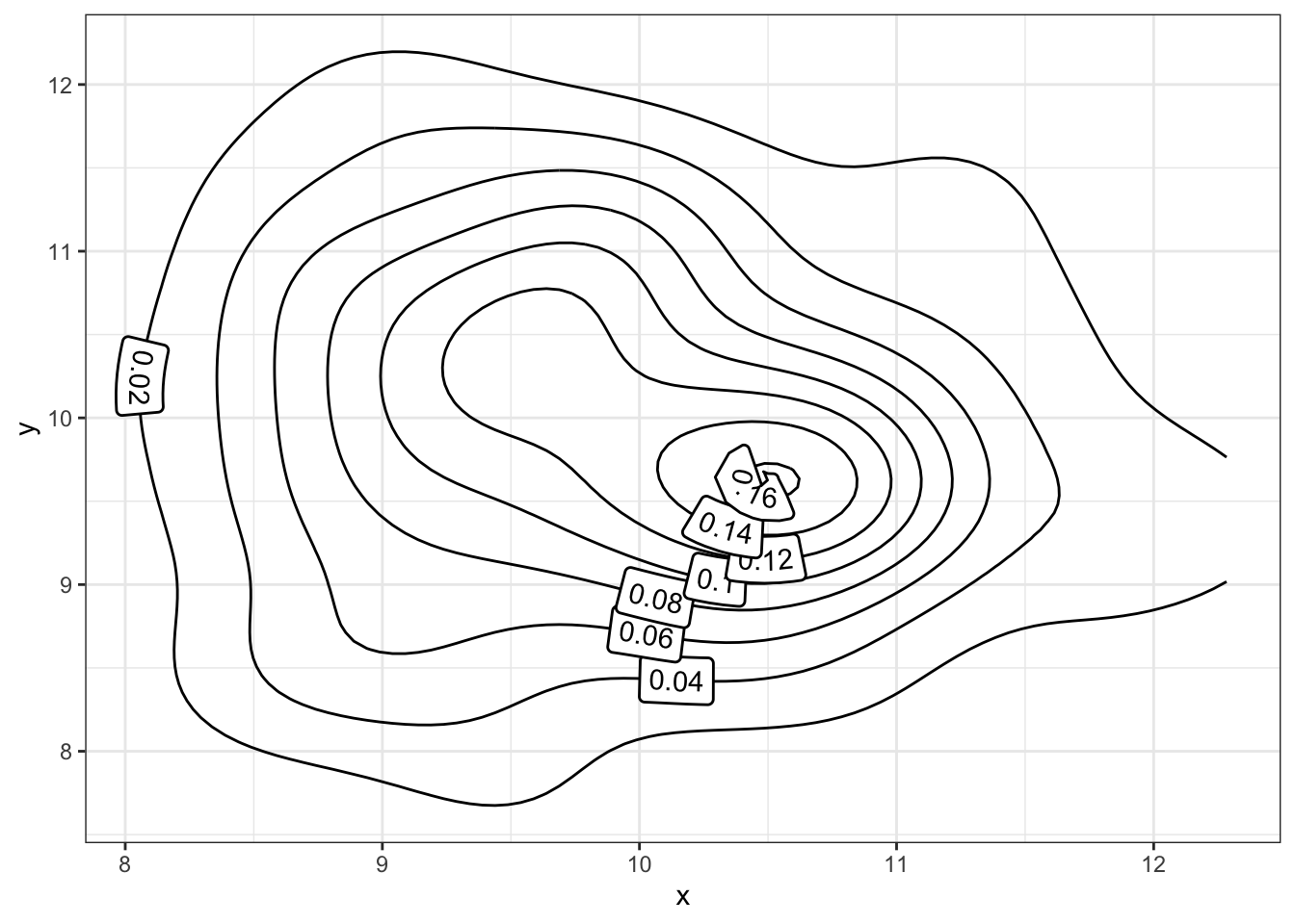
→ 2D density contours

2D density contours become now very easy to create with the geom_labeldensity2d() and geom_textdensity2d()

Example:

df = data.frame(x = rnorm(n=100, mean=10),
                y = rnorm(n=100, mean=10))

ggplot(df, aes(x, y)) + 
  geom_labeldensity2d() + theme_bw()


Contact

This document is a work by Yan Holtz. Any feedback is highly encouraged. You can fill an issue on Github, drop me a message on Twitter, or send an email pasting yan.holtz.data with gmail.com.

Github Twitter